What is a GNN?
For the use of IGNNITION, we focus on one of the most basic GNN architectures named Message-Passing Neural Networks (MPNN), which is a well-known GNN family that covers a wide range of standard GNN architectures.
The input of a GNN is a graph G=(V, E) – directed or undirected – that comprises a set of nodes \(V\) and some edges connecting them \(E\). Each node v has an associated vector of a predefined size that encodes its state, namely, the node hidden state \(h_v\). At the beginning of a GNN execution, hidden state vectors \(h_v\) are initialized with some node-related features \(x_v\) included in the input graph. Optionally, edges may also contain a set of features denoted by \(e_{uv}\) where \(u,v \in V\).
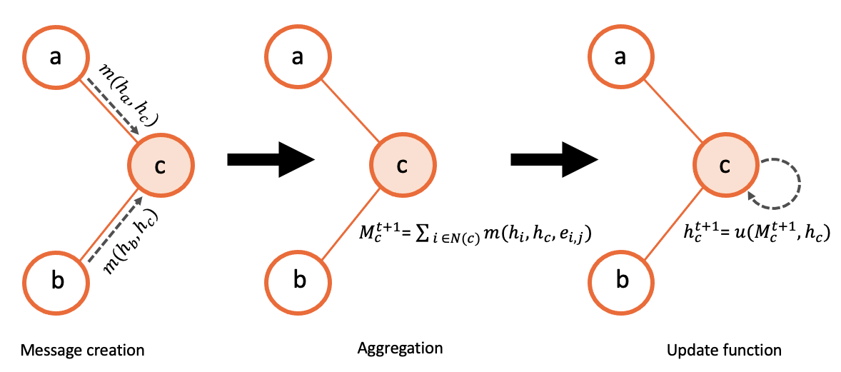
Once the hidden states are initialized, a message-passing algorithm is executed according to the connections of the input graph. In this message-passing process, three main phases can be distinguished: (i) Message, (ii) Aggregation, and (iii) Update. First, every node \(v \in V\) sends its hidden state to all its neighbors \(u \in N(v)\). Then, each node applies the message function \(M(·)\) to each of the received messages respectively, to obtain a new more refined representation of the state of its neighbors. After this, every node merges all the computed messages from its neighbors into a single fixed-size vector \(m_v\) that comprises all the information. To do this, they use a common Aggregation function (e.g., element-wise summation ). Lastly, every node applies an Update function \(U(·)\) that combines its own hidden state \(h_v\) with the final aggregated message from the neighbors to obtain its new hidden state. Finally, all this message-passing process is repeated a number of iterations \(T\) until the node hidden states converge to some fixed values. Hence, in each iteration, a node potentially receives — via its direct neighbors — some information of the nodes that are at \(k\) hops in the graph. Formally, the message passing algorithm can be described as:
All the process is also summarized in the figure below:
After completing the T message-passing iterations, a Readout function \(R(·)\) is used to produce the output of the GNN model. Particularly, this function takes as input the final node hidden states \(h^t_v\) and converts them into the output labels of the model \(\hat{y}\):
At this point, two main alternatives are possible: (i) produce per-node outputs, or (ii) aggregate the node hidden states and generate global graph-level outputs. In both cases, the Readout function can be applied to a particular subset of nodes.
One essential aspect of GNN is that all the functions that shape its internal architecture is universal. Indeed, it uses four main functions that are replicated multiple times along the GNN architecture: (i) the Message , (ii) the Aggregation , (ii) the Update , and (iv) the Readout . Typically, at least, and are modeled by three different Neural Networks (e.g., fully-connected NN, Recurrent NN) which approximate those functions through a process of joint fine-tunning (training phase) of all their internal parameters. As a result, this dynamic assembly results in the learning of these universal functions that capture the patterns of the set of graphs seen during training, and which allows its generalization over unseen graphs with potentially different sizes and structures.
Additional material
Some users may find the previous explanation too general as, for simplicity, we focus only on the most general scenario. For this reason, we provide some additional material to learn about GNNs in more depth.
Blogs
Below we also enumerate several blogs that provide a more intuitive overview of GNNs.
Courses
Due to the fact that GNNs are still a very recent topic, not too many courses have been taught covering this material. We, however, recommend a course instructed by Standford university named Machine learning with graphs.